Jensen's Inequality
·
Zach Ocean
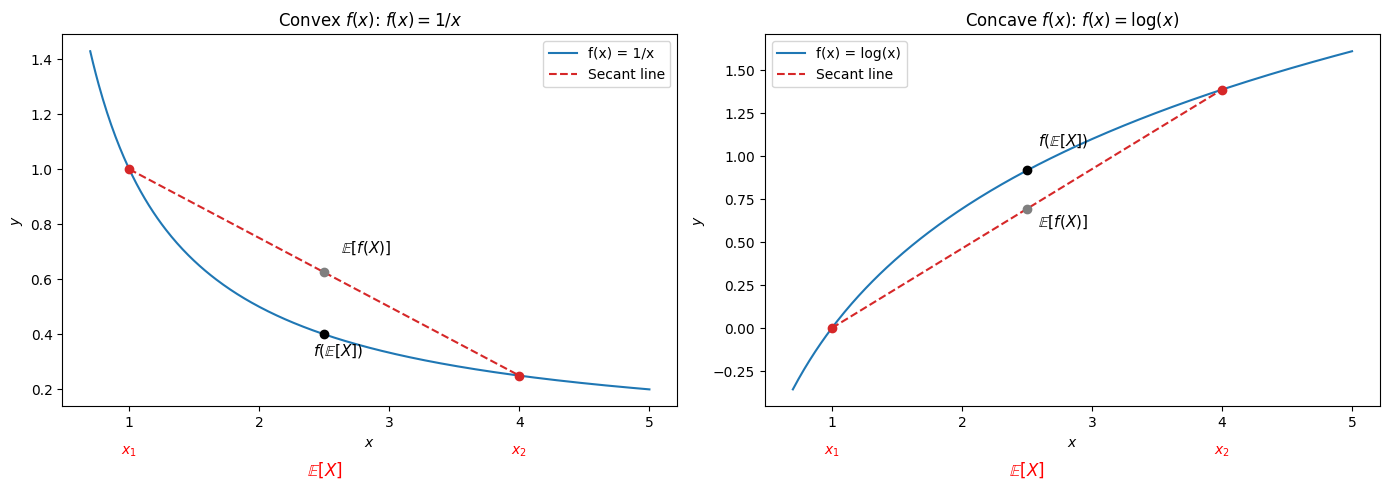
Jensens’ inequality says that for convex function and random variable , . (And conversely, for concave , the reverse relationship holds).
A good way to remember the direction of the inequality is by picturing the graphs below.
(Thanks to Cursor and Codex for help with the Matplotlib charts, code reproduced below.)
import matplotlib.pyplot as plt

import numpy as np

# Set up figure and axes
fig, axes = plt.subplots(1, 2, figsize=(14, 5))

# --- Convex Function: f(x) = 1/x, x > 0 ---
x1_c, x2_c = 1, 4
EX_c = (x1_c + x2_c) / 2
f_convex = lambda x: 1 / x

x_c = np.linspace(0.7, 5, 400)
ax = axes[0]
ax.plot(x_c, f_convex(x_c), label='f(x) = 1/x', color='C0')

# Secant line
f_x1_c, f_x2_c = f_convex(x1_c), f_convex(x2_c)
secant_slope_c = (f_x2_c - f_x1_c) / (x2_c - x1_c)
secant_c = lambda x: f_x1_c + secant_slope_c * (x - x1_c)
ax.plot([x1_c, x2_c], [f_x1_c, f_x2_c], 'C3--', label="Secant line")

# Points
ax.plot([x1_c, x2_c], [f_x1_c, f_x2_c], 'o', color='C3')
ax.plot(EX_c, f_convex(EX_c), 'ko')
ax.plot(EX_c, secant_c(EX_c), 'o', color="C7")

# Chart title and labels
ax.set_title("Convex $f(x)$: $f(x) = 1/x$")
ax.set_xlabel("$x$")
ax.set_ylabel("$y$")
ax.legend()

# Annotate x-axis labels after setting title/labels/legend to get correct ylim
ylim_c = ax.get_ylim()
y_min_c = ylim_c[0]
ax.annotate(r'$x_1$', (x1_c, y_min_c), textcoords="offset points", xytext=(0, -35), ha='center', color='red')
ax.annotate(r'$x_2$', (x2_c, y_min_c), textcoords="offset points", xytext=(0, -35), ha='center', color='red')
ax.annotate(r'$\mathbb{E}[X]$', (EX_c, y_min_c), textcoords="offset points", xytext=(0, -50), ha='center', fontsize=12, color='red')
ax.annotate(r'$f(\mathbb{E}[X])$', (EX_c, f_convex(EX_c)), textcoords="offset points", xytext=(-8, -15), ha='left', fontsize=11)
ax.annotate(r'$\mathbb{E}[f(X)]$', (EX_c, secant_c(EX_c)), textcoords="offset points", xytext=(12, 14), ha='left', fontsize=11)

# --- Concave Function: f(x) = log(x), x > 0 ---
x1_v, x2_v = 1, 4
EX_v = (x1_v + x2_v) / 2
f_concave = np.log

x_v = np.linspace(0.7, 5, 400)
ax = axes[1]
ax.plot(x_v, f_concave(x_v), label='f(x) = log(x)', color='C0')

# Secant line
f_x1_v, f_x2_v = f_concave(x1_v), f_concave(x2_v)
secant_slope_v = (f_x2_v - f_x1_v) / (x2_v - x1_v)
secant_v = lambda x: f_x1_v + secant_slope_v * (x - x1_v)
ax.plot([x1_v, x2_v], [f_x1_v, f_x2_v], 'C3--', label="Secant line")
ax.plot([x1_v, x2_v], [f_x1_v, f_x2_v], 'o', color='C3')

# Points
ax.plot(EX_v, f_concave(EX_v), 'ko')
ax.plot(EX_v, secant_v(EX_v), 'o', color="C7")

ax.set_title("Concave $f(x)$: $f(x) = \log(x)$")
ax.set_xlabel("$x$")
ax.set_ylabel("$y$")
ax.legend()

# Annotate x-axis labels after setting title/labels/legend to get correct ylim
ylim_v = ax.get_ylim()
y_min_v = ylim_v[0]
ax.annotate(r'$x_1$', (x1_v, y_min_v), textcoords="offset points", xytext=(0, -35), ha='center', color='red')
ax.annotate(r'$x_2$', (x2_v, y_min_v), textcoords="offset points", xytext=(0, -35), ha='center', color='red')
ax.annotate(r'$\mathbb{E}[X]$', (EX_v, y_min_v), textcoords="offset points", xytext=(0, -50), ha='center', fontsize=12, color='red')
ax.annotate(r'$f(\mathbb{E}[X])$', (EX_v, f_concave(EX_v)), textcoords="offset points", xytext=(8, 18), ha='left', fontsize=11)
ax.annotate(r'$\mathbb{E}[f(X)]$', (EX_v, secant_v(EX_v)), textcoords="offset points", xytext=(8, -13), ha='left', fontsize=11)

plt.tight_layout()
plt.show()